
Article by Dario Gozzi
Oscilloscopes are versatile electronic instruments commonly used by engineers to perform waveform and signal analysis in electronic circuits. By attaching probes to different points in a circuit, oscilloscopes can display and measure voltage waveforms, analyze signal integrity, troubleshoot circuit problems, and analyze signal frequency and phase. With the ability to capture and display electronic signals in real time, oscilloscopes are a vital tool for optimizing the performance of the circuits and ensuring they work as intended.
In particular, oscilloscopes should be easy to learn and use, helping you work at peak efficiency and productivity. This means being able to focus solely on the design, rather than the measurement tools.
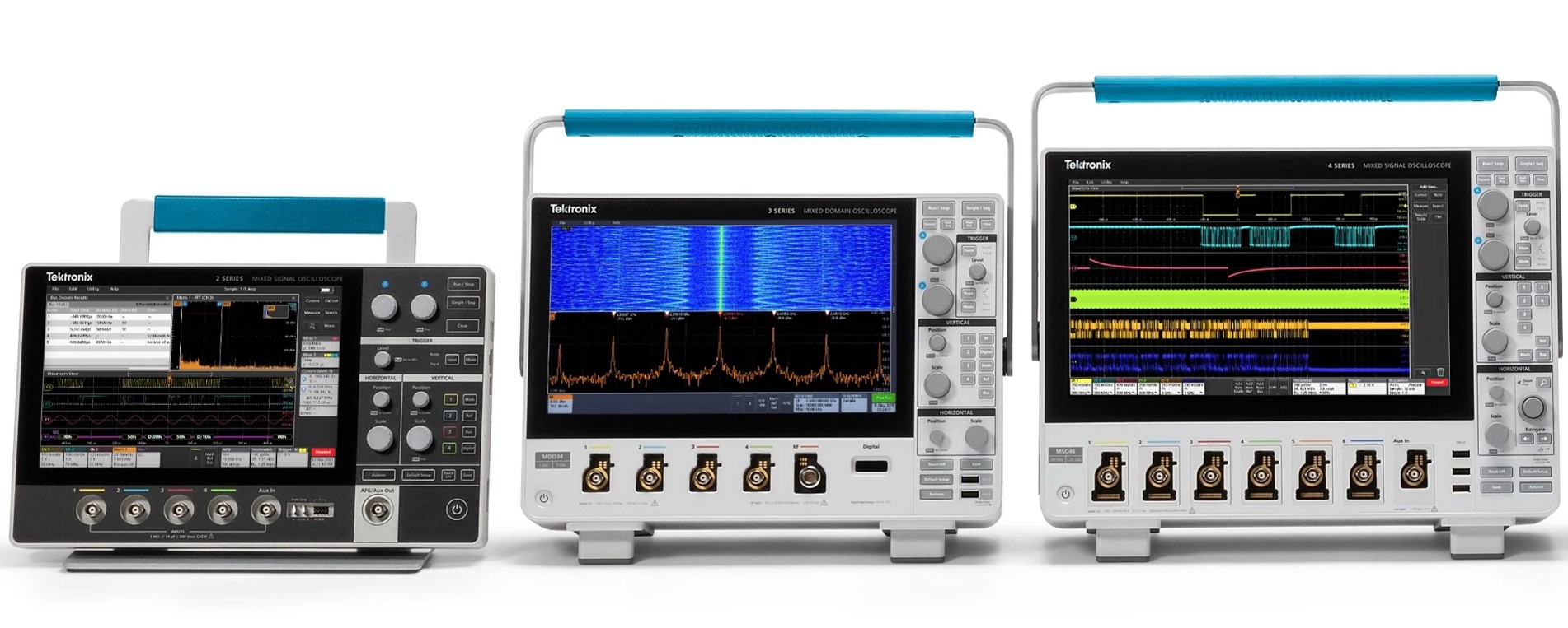
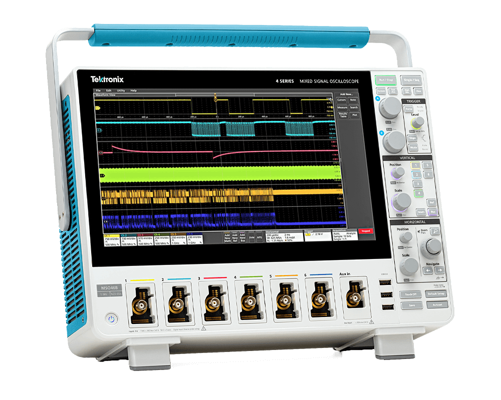
Just as there is no typical driver, there is no typical oscilloscope user. Regardless of whether you prefer a traditional instrument interface or a Windows software interface, it is important to have flexibility in how you operate your oscilloscope. Many oscilloscopes strike a balance between performance and simplicity by providing multiple ways to use the instrument. The front panel layout of a typical oscilloscope provides dedicated vertical, horizontal, and trigger controls.
Measurement probes
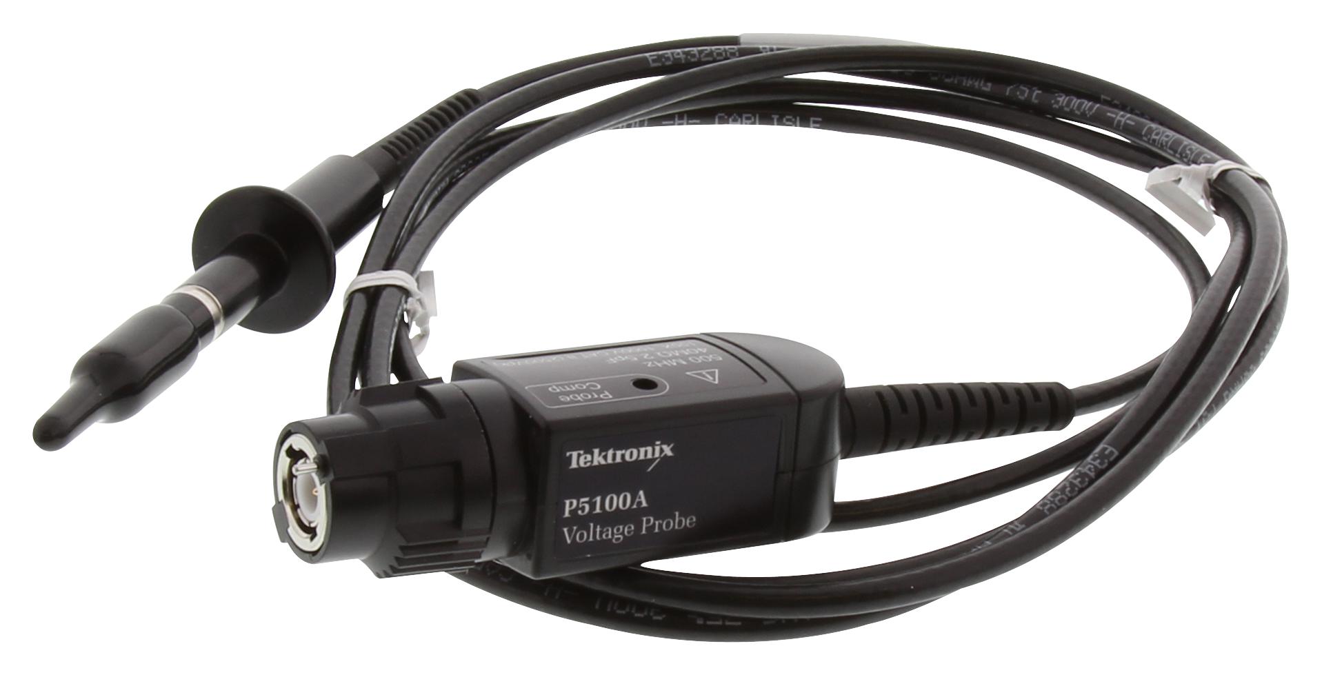
Even the most advanced instrument can only be as accurate as the data fed into it. A probe works with an oscilloscope as an integral part of the measurement system. Precision measurements start at the tip of the probe. The right probes matched to the oscilloscope and the device under test (DUT) not only bring the signal to the oscilloscope cleanly, but also amplify and preserve it for maximum signal integrity and measurement accuracy.
Besides, a probe establishes a physical and electrical connection between a test point or signal source and an oscilloscope. Depending on the measurement needs, this connection can be as simple as a piece of wire or as sophisticated as an active differential probe.
Whatever probe you use, it must provide a connection of adequate practicality and quality between the signal source and the oscilloscope input. In particular, the adequacy of the connection is defined by three key points: physical connection, impact on circuit operation, and signal transmission.
Bandwidth
Bandwidth determines the fundamental ability of an oscilloscope to measure a signal. In detail, as the frequency of the signal increases, the ability of an oscilloscope to accurately display the signal decreases. The bandwidth specification indicates the frequency range that the oscilloscope can accurately measure.
Besides, the bandwidth of the oscilloscope is specified as the frequency at which a sinusoidal input signal is attenuated to 70.7% of the true amplitude of the signal, known as the -3 dB point, a term based on a logarithmic scale.
Without adequate bandwidth, an oscilloscope cannot resolve changes in the signal that occur at high frequencies: the amplitude is distorted, edges disappear, details are lost. All the functionality of the oscilloscope would be lost.
Some oscilloscopes provide a method of improving the bandwidth through digital signal processing (DSP). A DSP arbitrary equalization filter can be used to improve the oscilloscope channel response. This filter extends the bandwidth, flattens the channel frequency response, improves phase linearity, and provides better channel matching. It also reduces the rise time and improves the step response in the time domain.
Rise time
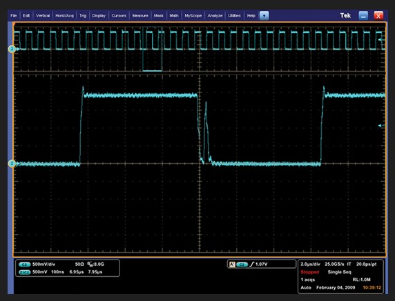
Rise time describes the useful frequency range of an oscilloscope. Its measurements are critical in the digital world. Rise time may be a more appropriate performance consideration when you plan to measure digital signals, such as pulses and steps. In particular, an oscilloscope must have a sufficient rise time to accurately capture the details of fast transitions.
An oscilloscope with a very fast rise time will more accurately capture the critical details of fast signal transitions.
In some applications, you may only know the rise time of a signal. A constant allows you to relate the bandwidth and rise time of the oscilloscope using this equation:
bandwidth = K/rise time
Where K is a value between 0.35 and 0.45, depending on the shape of the oscilloscope’s frequency response curve and the rise time response of the pulse. Oscilloscopes with a bandwidth <1 GHz typically have a value of 0.35, while oscilloscopes with a bandwidth >1 GHz typically have a value between 0.40 and 0.45.
Sample rate
The sample rate is specified in samples per second (S/s). It defines the rate at which a digital oscilloscope takes a snapshot or sample of the signal, similar to frames in a movie. The faster an oscilloscope samples (that is, the higher the sample rate), the greater the resolution and detail of the displayed waveform, and the less likely it is that critical information or events will be missed.
The minimum sample rate can also be important if you need to observe slowly changing signals over long periods of time. Typically, the displayed sample rate changes as you adjust the horizontal scale control to maintain a constant number of waveform points in the displayed waveform record.
The method for calculating sample rate requirements varies based on the type of waveform you are measuring and the signal reconstruction method your oscilloscope uses.
To accurately reconstruct a signal and avoid aliasing, the Nyquist theorem states that the signal must be sampled at least twice as fast as its highest frequency component. This theorem, however, assumes an infinite record length and a continuous signal. Since no oscilloscope offers an infinite record length, and glitches are not continuous by definition, sampling at only twice the highest frequency component is usually insufficient.
In reality, accurately reconstructing a signal depends on both the sampling rate and the interpolation method used to fill in the gaps between samples. Some oscilloscopes allow you to select sin(x)/x interpolation for measuring sinusoidal signals, or linear interpolation for square waves, pulses, and other signal types.
For accurate reconstruction using sin(x)/x interpolation, the oscilloscope should have a sampling rate of at least 2.5 times the highest frequency component of the signal. Using linear interpolation, the sampling rate should be at least 10 times the highest frequency component of the signal.
Some measurement systems with sampling rates up to 10 GS/s and bandwidths up to 3+ GHz are optimized to capture very fast, single, transient events by oversampling up to 5 times the bandwidth.
Record length
Record length, expressed as the number of points that make up a complete waveform recording, determines the amount of data that can be acquired with each channel. Because an oscilloscope can only store a limited number of samples, the duration of the waveform (time) is inversely proportional to the oscilloscope’s sampling rate.
Oscilloscopes allow you to select the record length to optimize the level of detail needed for your application. If you are analyzing a very stable sinusoidal signal, you may only need a record length of 500 points, but if you are isolating the causes of timing anomalies in a complex digital data stream, you may need a million points for a given record length.
Performance that increases measurement potential
The complexity of an oscilloscope has several attributes that you need to know to master it and get the most out of it.
Frequency response
Bandwidth alone is not enough to ensure that an oscilloscope can accurately capture a high-frequency signal. In particular, the goal of oscilloscope design is a specific type of frequency response: maximally flat envelope delay (MFED). This type of frequency response provides excellent pulse fidelity with minimal overshoot and ringing (the oscillation of a signal, especially in step response). Since a digital oscilloscope is made up of real amplifiers, attenuators, ADCs, interconnects, and relays, the MFED response is a goal that can only be approached. Pulse fidelity varies greatly by model and manufacturer.
Vertical sensitivity
Vertical sensitivity indicates how much the vertical amplifier can amplify a weak signal. It is generally measured in millivolts (mV) per division. The smallest voltage detected by a general purpose oscilloscope is typically about 1 mV per vertical division of the screen.
Sweep rate
The sweep rate is how quickly the trace can sweep across the oscilloscope screen, making it possible to see fine detail. The sweep rate of an oscilloscope is represented by time (seconds) per division.
Gain accuracy
This is how accurately the vertical system attenuates or amplifies a signal, generally represented as a percentage error.
Horizontal accuracy (time base)
Horizontal accuracy, or time base accuracy, is how accurately the horizontal system displays the timing of a signal, generally represented as a percentage error.
Vertical resolution (analog-to-digital converter)
The vertical resolution of the analog-to-digital converter (ADC), and therefore the digital oscilloscope, is how accurately it can convert input voltages into digital values. Vertical resolution is measured in bits. Computational techniques can improve the effective resolution, as exemplified by the high resolution acquisition mode.
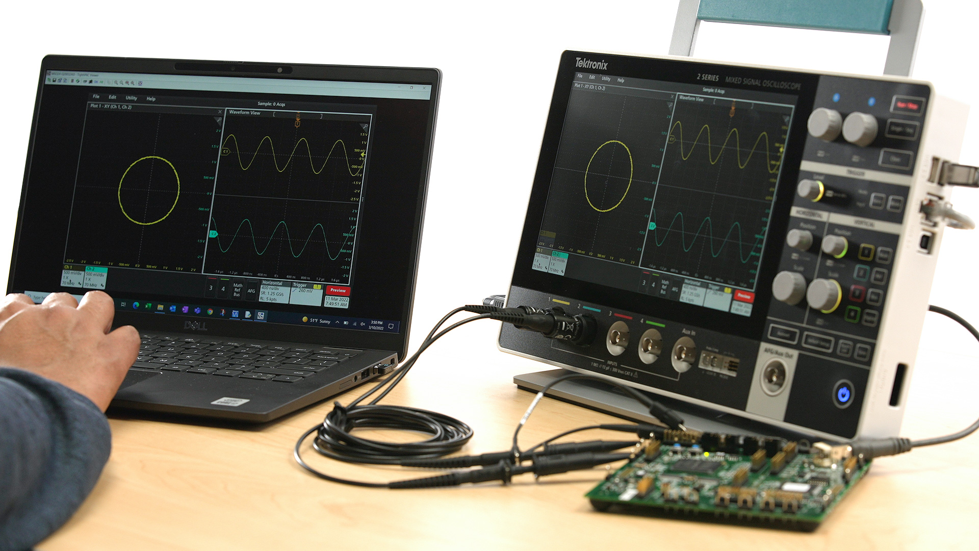
Connectivity
The need to analyze measurement results remains critical, as does the need to document them, sharing information easily and frequently. The connectivity of a modern oscilloscope offers advanced analysis capabilities and simplifies the documentation and sharing of results. Standard interfaces (GPIB, RS-232, USB and Ethernet) and network communication modules allow some oscilloscopes to offer a wide range of functionality and control. Some advanced oscilloscopes also allow you to create, edit and share documents while working with the instrument in your operating environment, access printing and file sharing resources over the network, and run third-party analysis software.


